Explorer

The Explorer is an experimental floating multi-tab dock for higher-level visual summaries across annotations, staging, signals, and output tables. Features may be added, changed, or refined over time.

Open it from the View menu or press Ctrl/Cmd-E.

Tabs

The Explorer includes several tabs:

• Harmonizer : project-wide summaries of signal and annotation naming across the current sample list

• Annotations : cohort-level summaries and direct overlap analyses across the current sample list or a compiled cache

• Hypnoscope : summaries of staging across all individuals in the current sample list (or cached)

• Waveforms : event-locked visualizations of signals for the current attached recording

• Tables : descriptive summary tables from the current output tables

• Plotter : plots of the current output dock

• Assoc : group-level association workflows for phenotypes, signals, and covariates

• Filter Design : interactive filter-design and response-plotting tools

• Topo : experimental topographic displays for channel-level summaries

Harmonizer

The Harmonizer tab provides project-wide summaries of signal and annotation naming across the current sample list. It is intended to help identify inconsistent labels before running cohort-level analyses.

Annotations

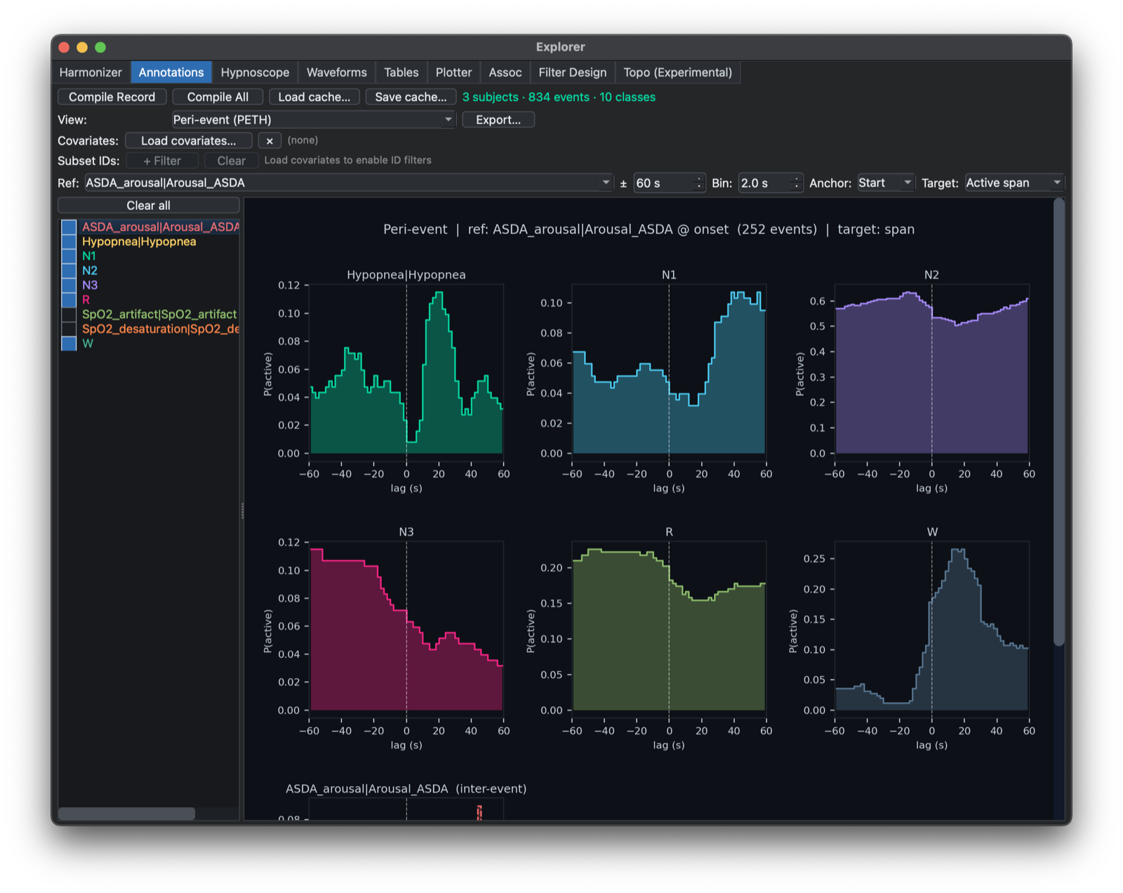
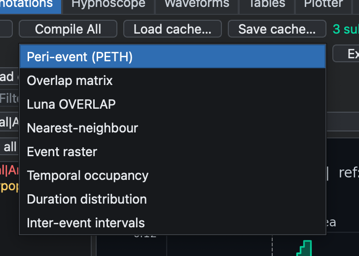
The Annotations tab compiles annotations across the whole sample list and supports several cohort-level views:

In addition to compiling across the project, the tab can choose a reference annotation class and adjust the analysis window, histogram bin width, and raster gap.

The Annotations tab supports compiled-cache save/load and figure export. For compiled cohort caches, Lunascope can also merge an external covariate table that contains an ID column. Low-cardinality columns from that table can then be used as ID-level filters, making it easier to restrict the cohort to a subgroup before plotting or computing summary statistics.

OVERLAP

The Luna OVERLAP mode exposes the native Luna OVERLAP analysis from within the Explorer. You provide the OVERLAP arguments directly in a free-text box, and choose whether to run on the current subject or on a compiled cohort timeline assembled from the current cache or sample list. In compiled-cohort mode, Lunascope concatenates individuals onto a non-overlapping synthetic timeline and inserts subject-boundary markers so background-restricted permutations still operate within person.

All returned Luna output tables are pushed to the standard Outputs dock. This makes it possible to inspect the full OVERLAP result set, including the usual seed-seed and seed-other summary tables, while keeping the setup inside the annotation workflow.

Hypnoscope

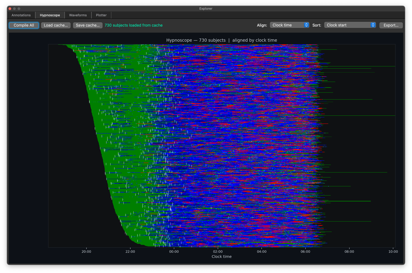
The Hypnoscope tab compiles staging annotations across the full sample list and renders a cohort hypnogram grid.

It supports project-wide compilation, alignment by Clock time, Elapsed recording, or Elapsed sleep, and sorting by alphabetical order, clock start, sleep efficiency, TST, or sleep-onset latency. This is intended as a compact cohort-level overview of staging timing and structure.

The Hypnoscope tab supports staging-cache save/load and figure export.

Waveforms

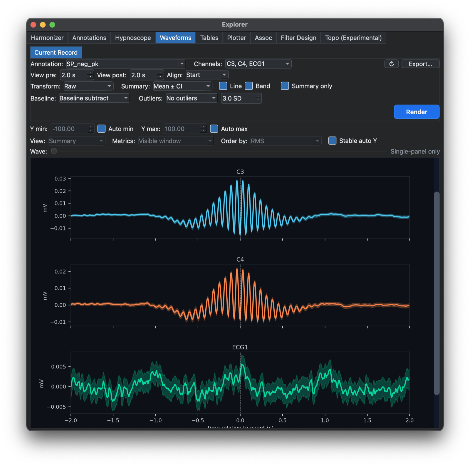
The Waveforms tab extracts peri-event signal windows from the currently attached record. You choose an annotation class, one or more EDF channels, pre-event and post-event windows, alignment to event Start, Midpoint, or Stop, and whether to baseline-subtract each extracted trace. The resulting display overlays individual traces together with a mean trace and confidence interval summary.

For single-record analyses, the tab also supports optional outlier handling on extracted traces. Outlying windows can either be left as is, winsorized, or removed entirely using a user-selected SD-based threshold.

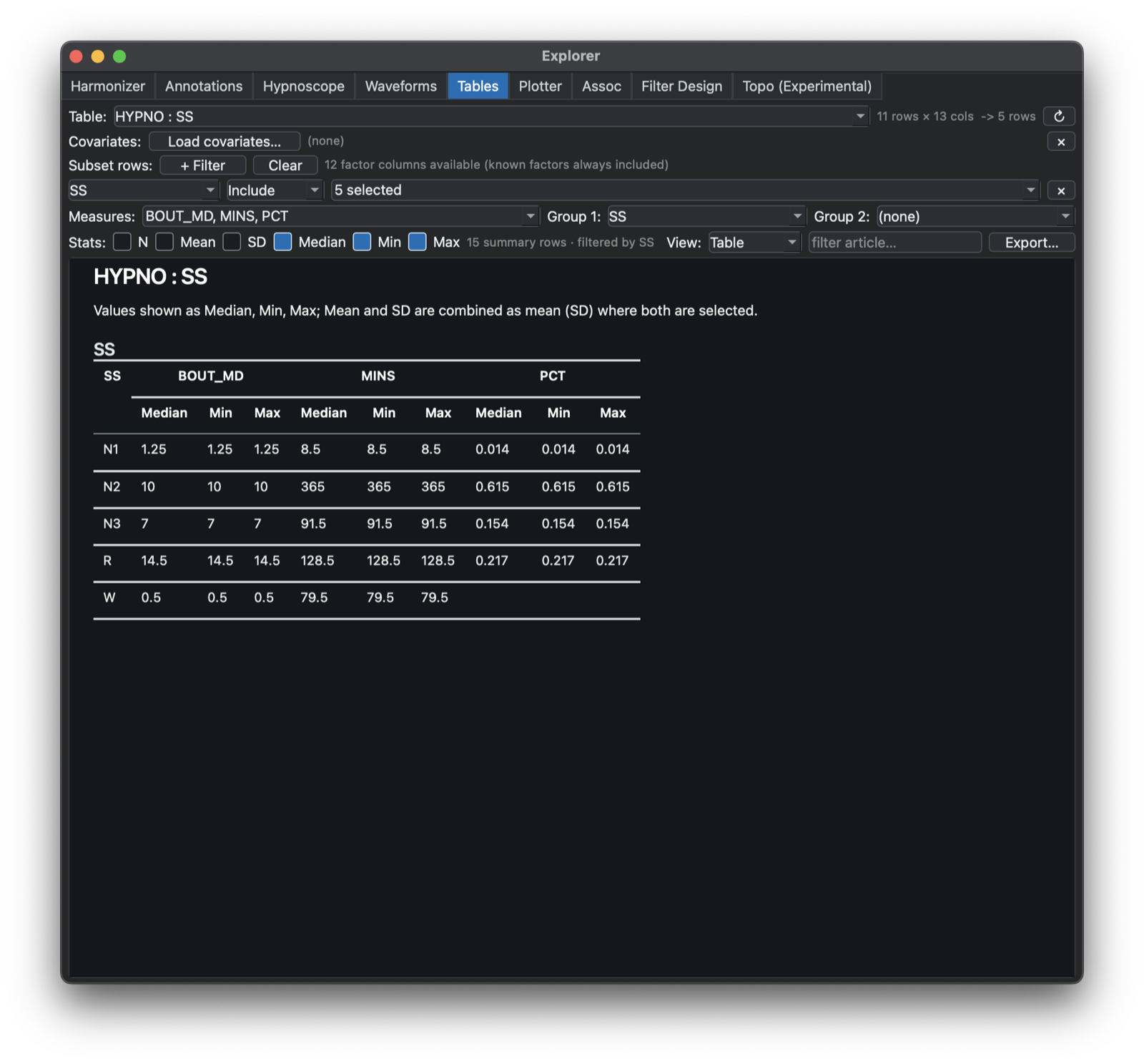
Tables

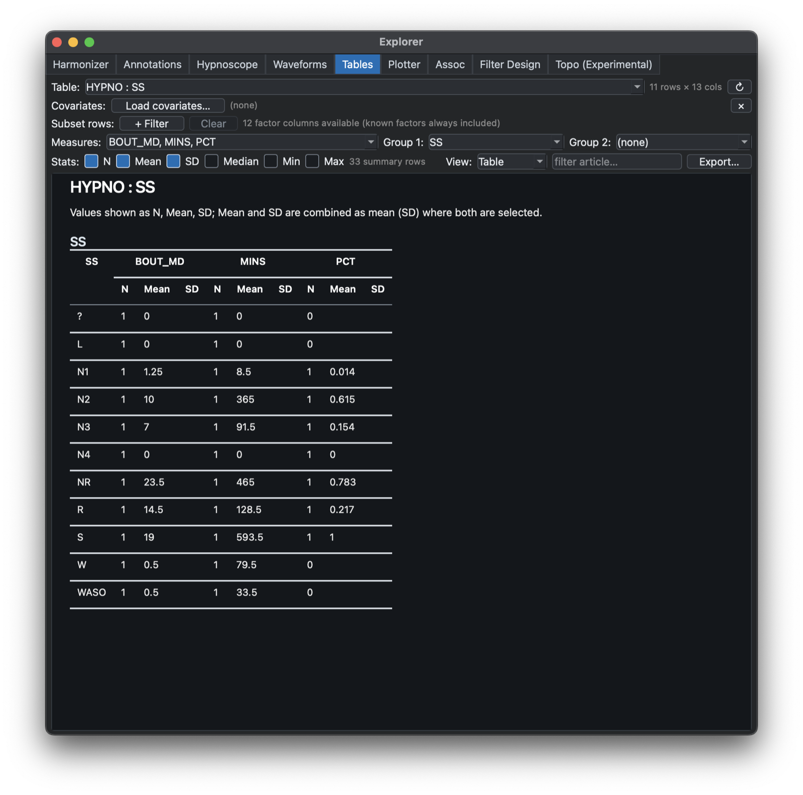
The Tables tab summarizes numeric columns from output tables. It supports selecting one or more measures, optional grouping by one or two factors, row filters, covariate-file merging, selectable summary statistics, and either grid-style or publication-style table output, as below.

Plotter

The Plotter tab turns output tables from the Outputs dock into figures. It supports auto-selected or explicit plot types (scatter, line, bar, histogram, box), X and Y variable selection, optional log scaling on either axis, two grouping variables, and either Overlay or Separate display for each grouping variable. It can also merge an external TSV/CSV covariate file as long as that file contains an ID column.

A row-subsetting control can be used to filter the current output table before plotting. This is useful when a Luna output contains multiple strata or analysis passes but only a subset should be shown in the figure.

When an X-axis factor looks numeric, the Plotter sorts it numerically rather than lexicographically. This avoids orderings such as 1, 10, 11, 2, 3 when plotting epoch numbers, bins, lags, or similar indexed variables.

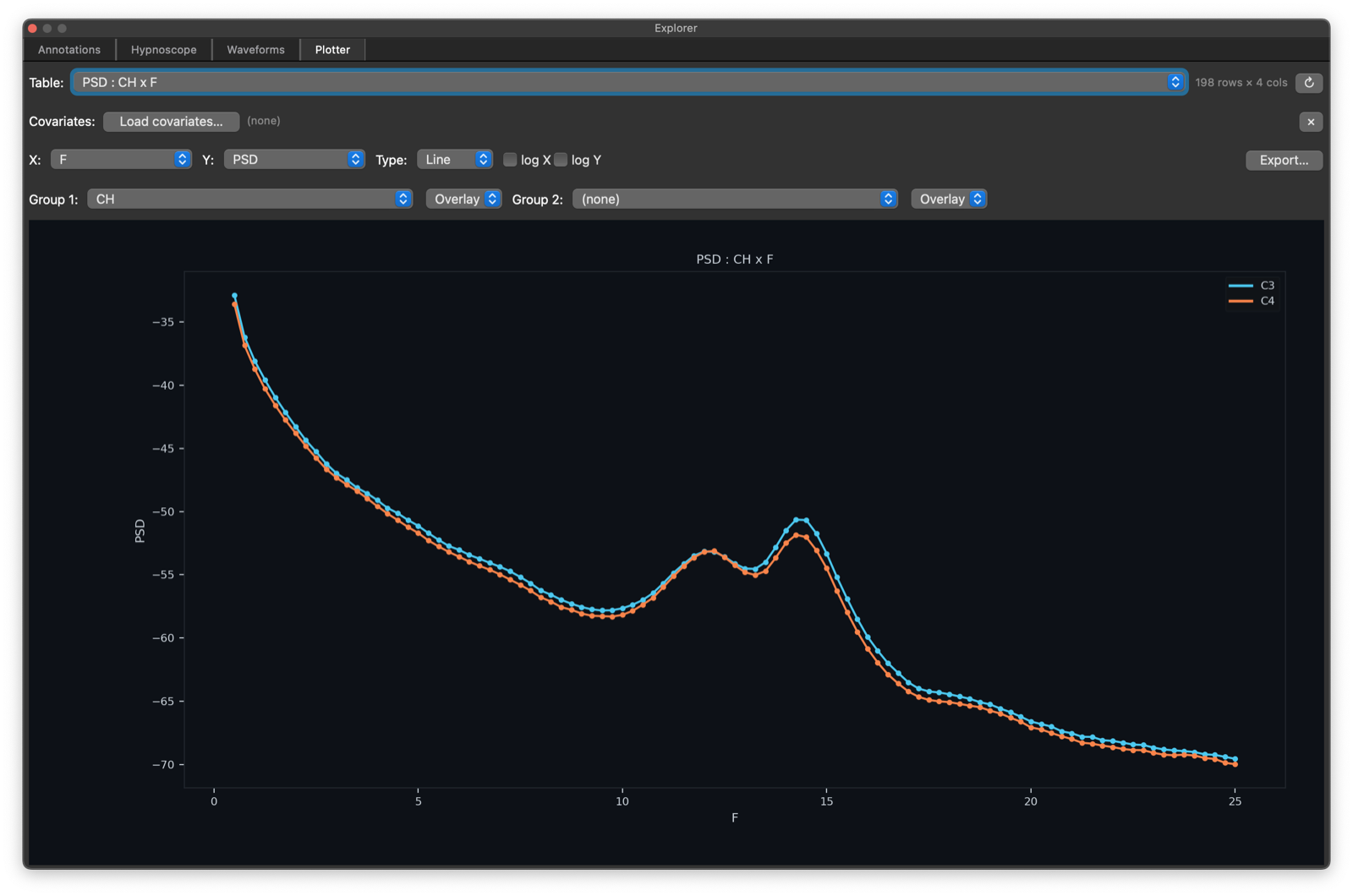
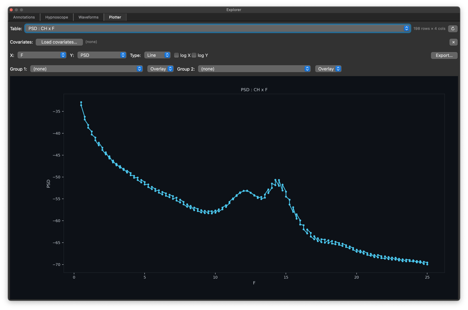
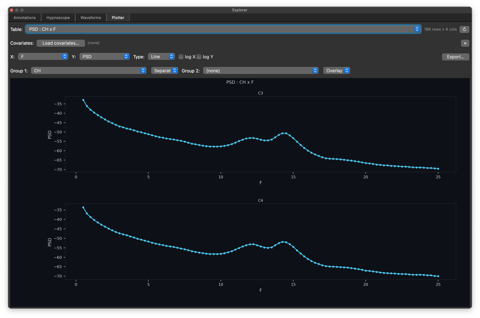
Note, when first loading a stratified table, for example by channel, the initial plot will combine all strata: here channels are interleaved effectively:

Selecting the CH to be the Group 1 stratifier yields a plot with two lines, one per unique value of CH (as above). You can also select Separate instead of Overlap to get multi-panel representations of the same data:

Assoc

The Assoc tab is for group-level association workflows that combine phenotypes, signal-derived measures, and covariates. It is intended for project-level analyses after relevant output tables and covariate data have been assembled. This is primarily an interface to Luna's GPA command.

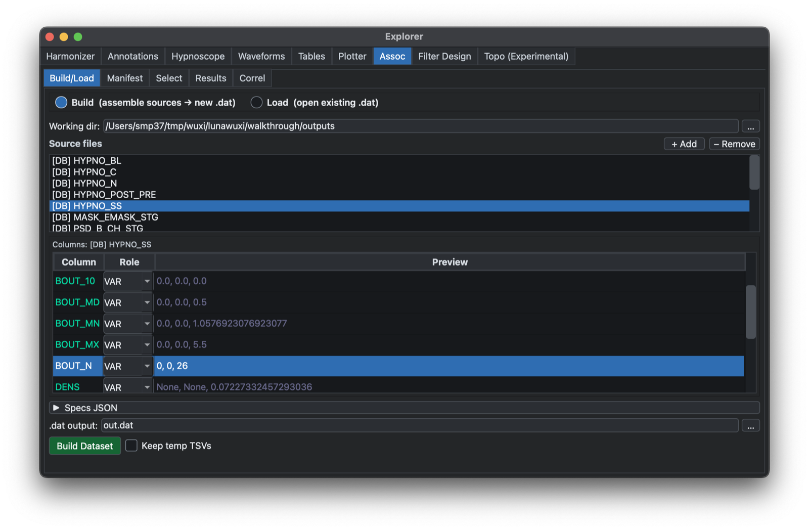
The image above shows how saved outputs ( e.g. TSV files with covariate data, or previously saved Outputs docks) can be selected. Each table is previewed; individual tables can be dropped. If loading from saved Outputs docks, Lunascope will know which variables are factors (FAC, e.g. channel or frequency or sleep stages, etc) and which are the core values ( e.g. here BOUT_N etc).

Having selected Build Dataset, a binary .dat file will be generated and a Manifest shown: here all values are expanded into a wide-formatted dataset.

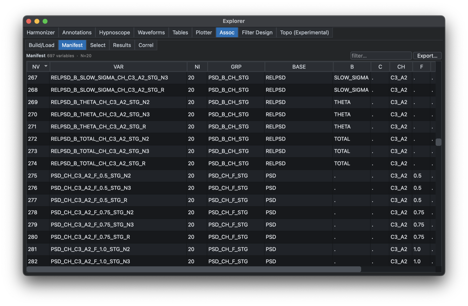
That is, if BOUT_N is defined for N1, N2, N3, etc, the generated dataset will have variables named BOUT_N_SS_N1, BOUT_N_SS_N2, BOUT_N_SS_N3 etc. The manifest (which can be saved) provides a convenient linking of long-to-short variable names and factor/level strata information.

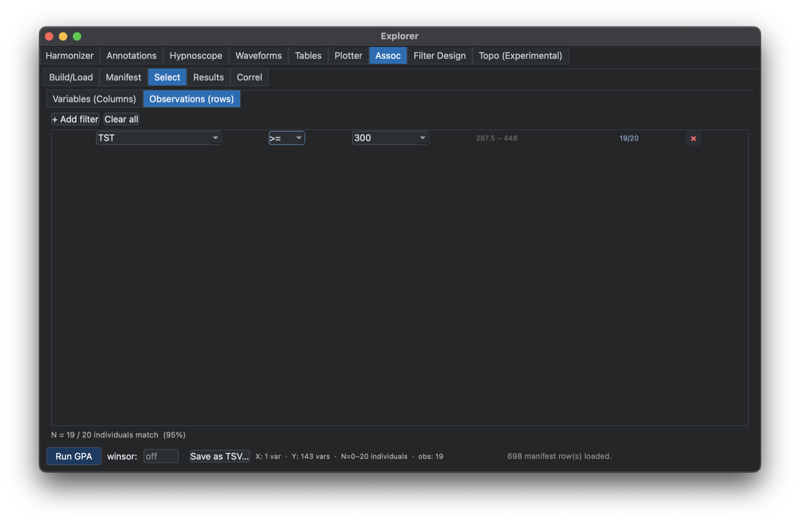
Next, one can Select which variables are dependents (Y), predictors (X) or covariates (Z), with this tab:

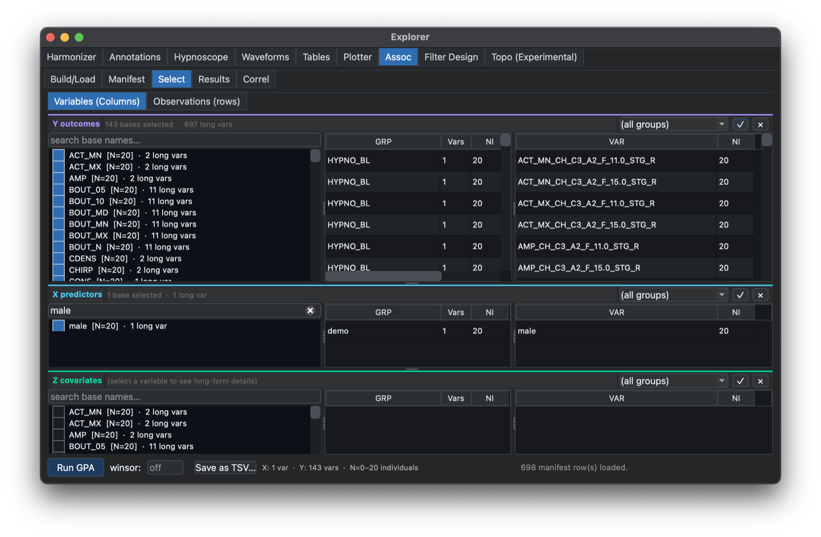
This tab also allows for selection of individuals, e.g. to specify subsets of the sample for analysis (e.g. here requiring at least 300 minutes of total sleep time (TST):

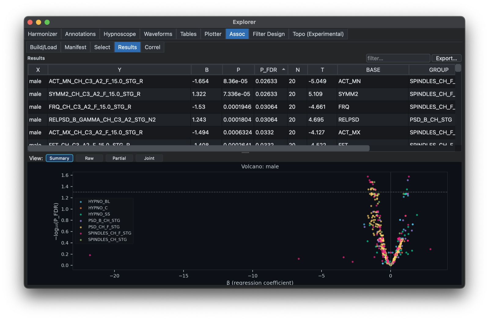
Having selected the variables and individuals for analysis, clicking Run GPA should bring up this view, with a table showing the results for each X/Y variable pair, and a volcano plot at the bottom:

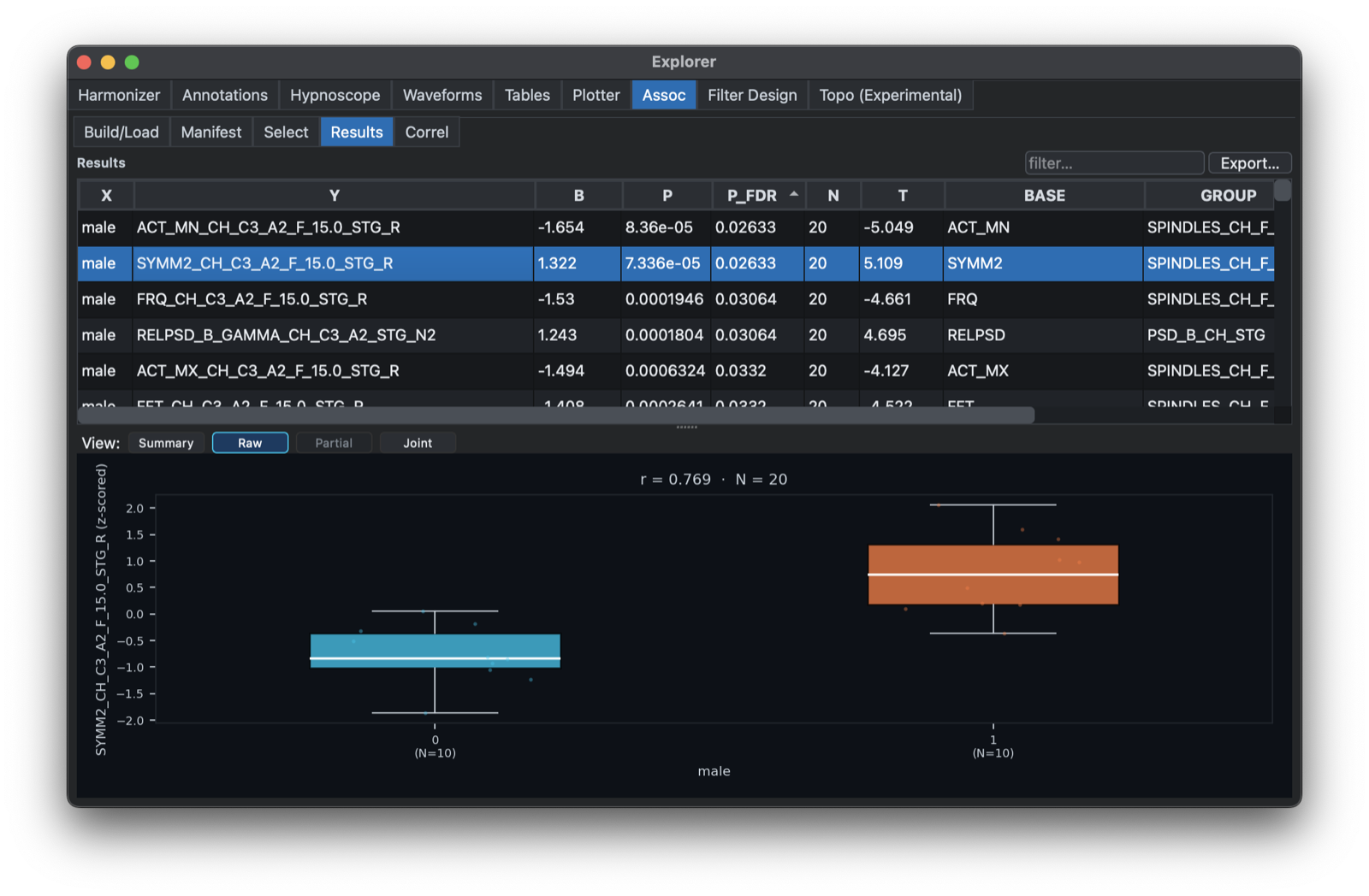
Clicking on a single row should bring up a scatter plot or box plot (depending on whether X is binary or continuous):

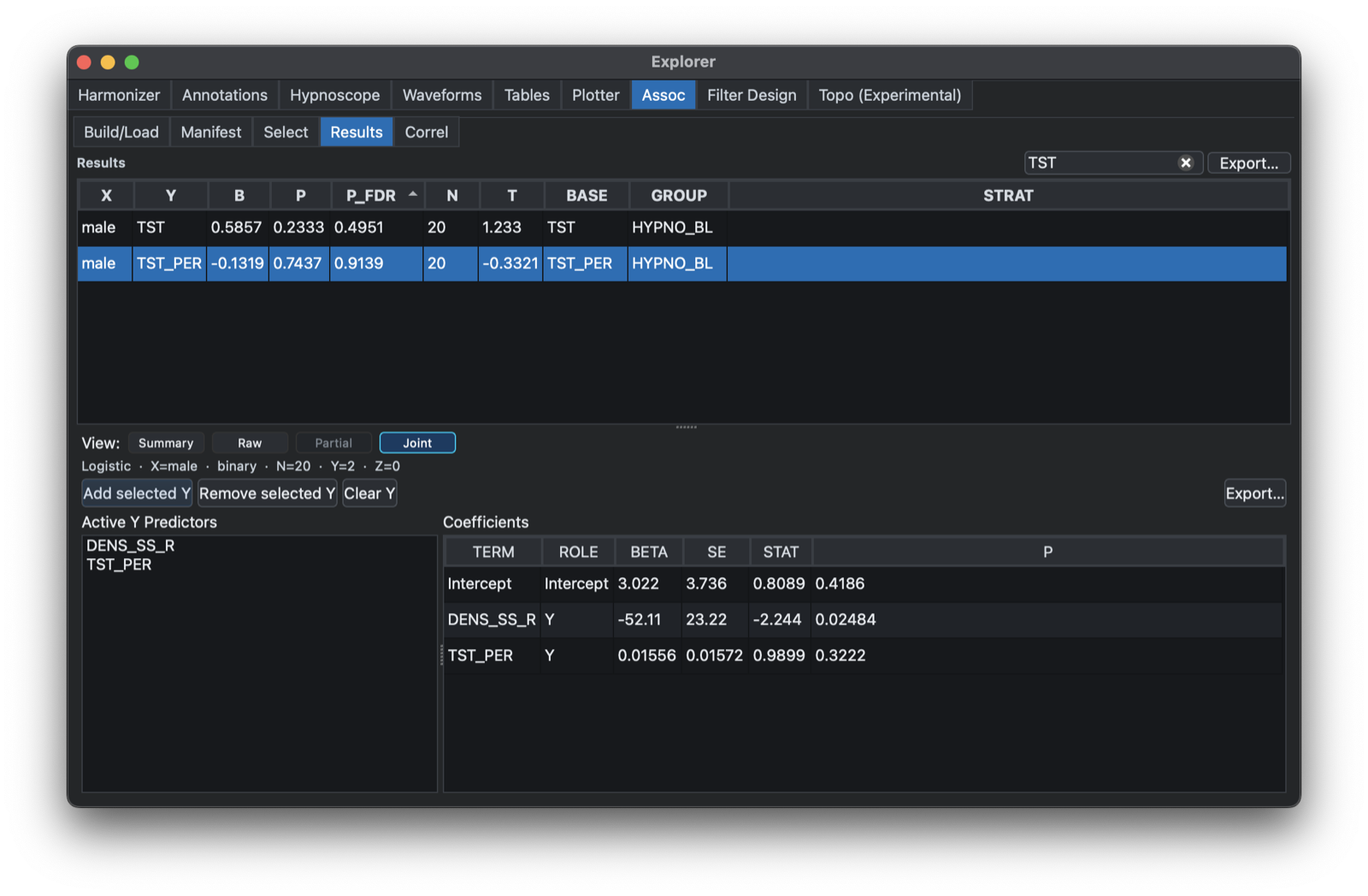
Selecting Joint allows for the creation of joint models, where multiple sleep metrics can be jointly modelled (note: here the model is reversed, such that X is the outcome in either a linear or logistic regression, allowing for one or more sleep metrics (conventionally denoted Y here) along with covariates. For example, here we ask whether REM density (minutes per hour of recording time) is associated with male sex (X=1), controlling for total persistent sleep time:

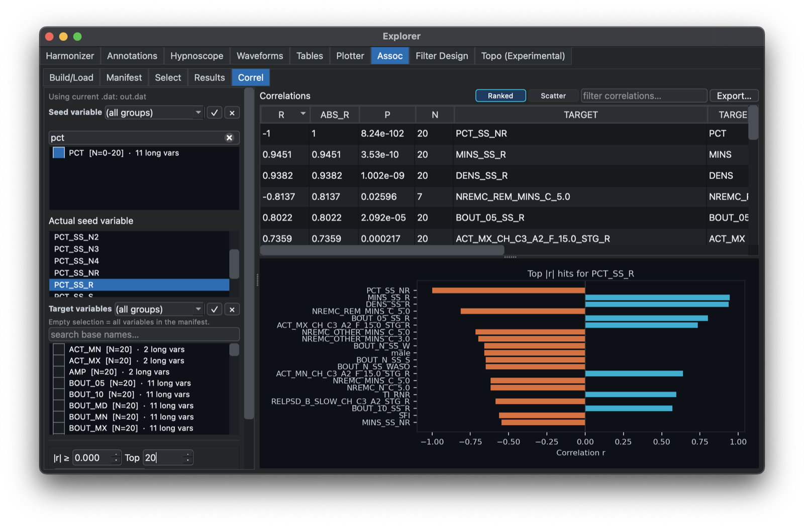
Finally, the Correl tab allows one to select a seed variable and see a quick (unconditional) plot of which other variables correlate strongly:

Filter Design

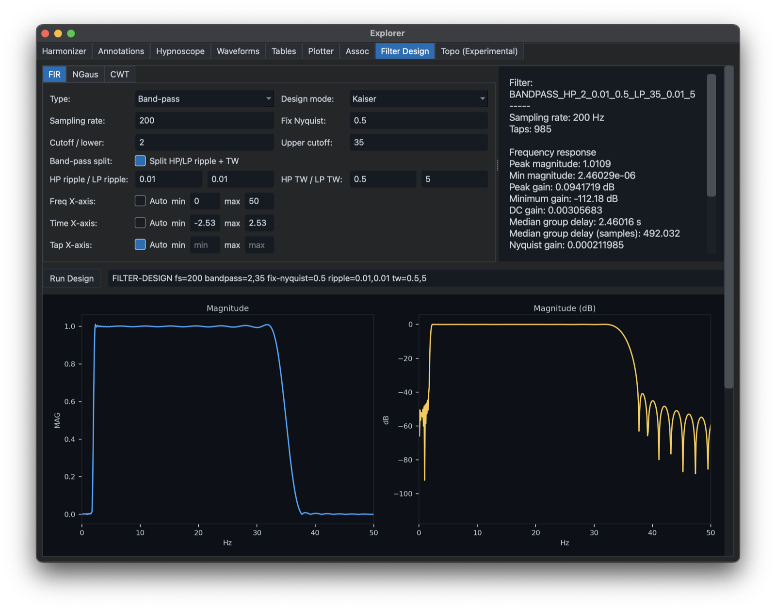
The Filter Design tab builds and visualizes filter specifications before they are used in scripts or configuration files. It supports FIR, CWT, and narrow Gaussian designs, with response plots, command text.

Topo

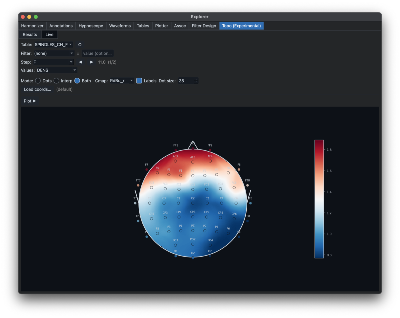
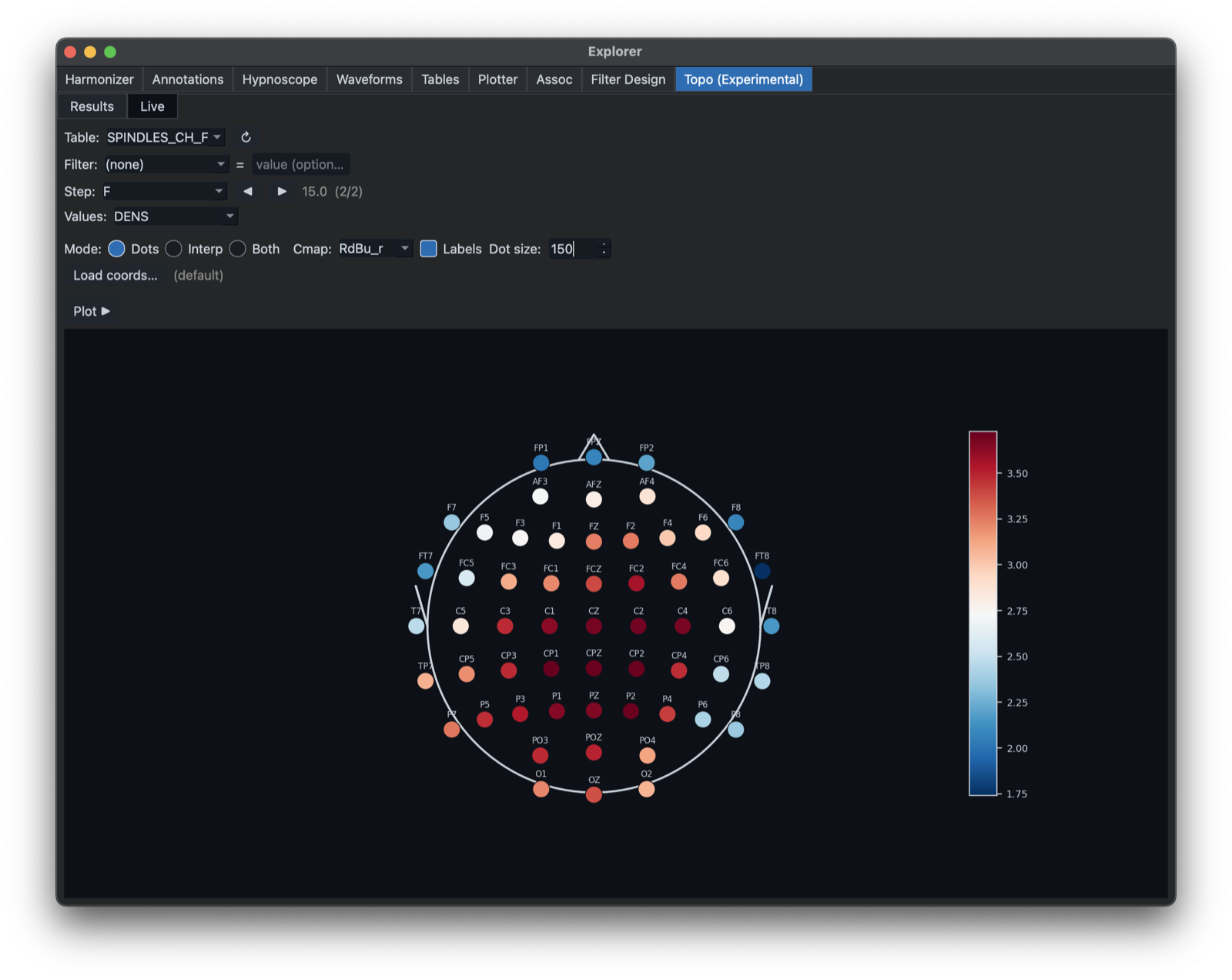
The Topo tab provides experimental topographic displays for channel-level summaries. It is intended for visualizing spatial patterns across compatible high-density EEG channel layouts.

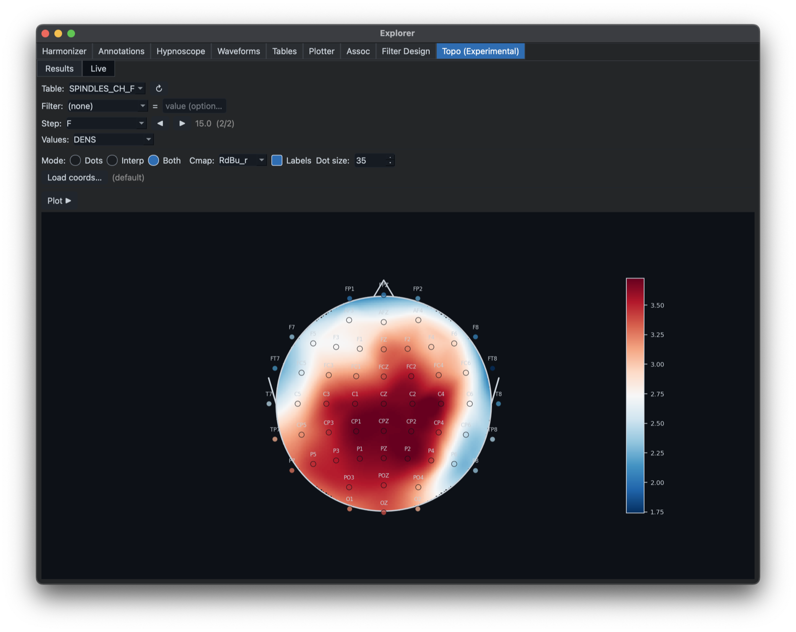
Inputs are selected from the current Outputs dock (note that one can load any TSV into the Outputs dock too, as well as capturing Luna command evaluations there). Above, we plot spindle density with a Step that looks at the F variable (11 or 15 Hz, for slow and fast spindles, respectively -- see Luna tutorial for more examples and context). Here are the values for fast spindles -- i.e. clicking the right arrow to get 15:

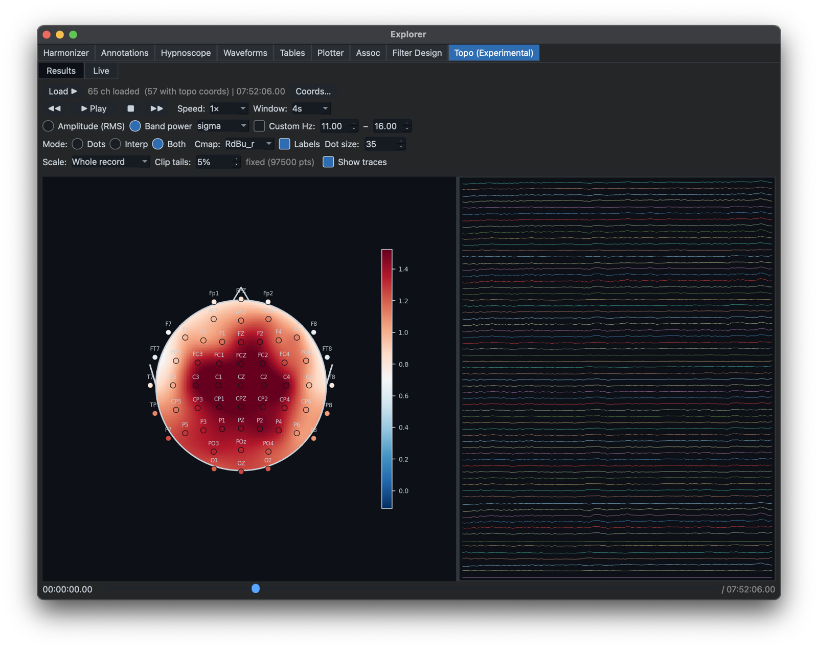
One can alter the appearance, for example removing the interpolated component:

Finally, there is an experimental player that can show spectral power or signal RMS continuously vary over time, by pressing the Play button.

---

Previous: Actigraphy | Next: Configuration